6.1 Unit 6: Integration and Accumulation of Change
4 min read•january 7, 2023
AP Calculus AB/BC ♾️
279 resourcesSee Units
Unit 6: Integration and Accumulation of Change
6.1: Exploring Accumulations of Change
Now that you have mastered derivatives, it’s time to explore another major concept in calculus, the integral. In our study of derivatives, we learned that the graph of a derivative shows the rate of change of the function. If we find the area between such a graph and the x-axis, that area gives the accumulation of change for the function.
To calculate this accumulation of change, we’ll use basic geometry area skills: rectangles, circles, triangles, and trapezoids. Let’s say we have a function, g(x), which has a derivative, f(x), as shown below.
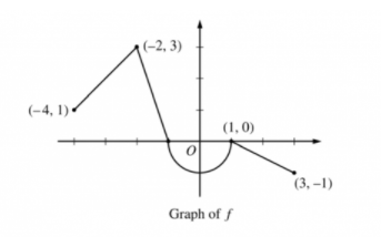
Image Courtesy of Albert.io
To find

we will add up the area between the derivative graph and the x-axis over the interval from 0 to 3 (the lower number on the integral symbol defines the starting point).
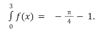
The region from x = 0 to x = 1 is a quarter of a circle with a radius of 1. That means it has an area of π/4. However, we have to be mindful of the sign of the areas when evaluating integrals this way. As we move along the x-axis to the right, the sign of the x-portion of the area is positive. If the derivative graph is below the x-axis, the y-portion of the area is negative. In this case, our answer should be -π/4 because positive (x-portion) times negative (y-portion) is negative. Similarly, from x = 1 to x = 3 we have a right triangle. Our x-portion is positive and our y-portion is negative. Using the formula for the area of a triangle we have 12(2)(-1)= -1. Adding this to the area from the previous interval, we have
If we move to the left along the x-axis, the x-portion of the area becomes negative. If the derivative graph is above the x-axis, the y-portion of the area is positive. For example, to find
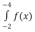
the x-portion of the trapezoid area is negative and the y-portion is positive.

Note About Units: The units for this type of accumulation problem can be found by multiplying the units for y by the units for x.
6.2 Approximating Areas with Riemann Sums
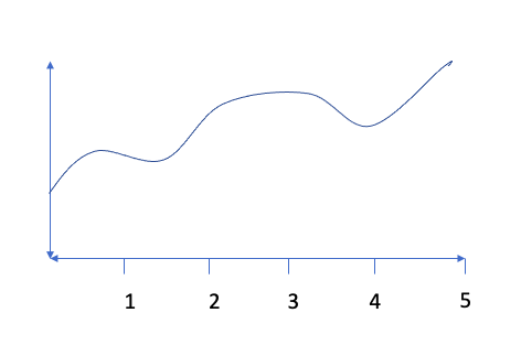
Another way to approximate the area under a curve (i.e., an integral), is to use the area of rectangles or trapezoids using something called a Riemann Sum. Let’s say we have the function, f(x), graphed below.
The true value of
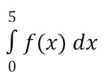
would give us the exact area under the curve (between the function and the x-axis). However, we are unable to use the shapes we used in the previous section to find this exact area. That’s where Riemann comes in handy!
There are 4 different types of Riemann Sums: right, left, mid-point, and trapezoid. These types of problems specify how many sub-intervals to use (i.e., how many rectangles or trapezoids to create). For this example, let’s assume we are asked to use 5 equal subintervals to estimate the value of

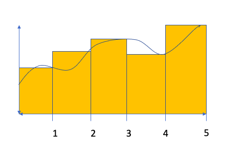
For a right Riemann Sum, we would create five equally-sized bases for rectangles using x-lengths of 1 (e.g. the length from 0 to 1 would be the base of the first rectangle). Then, we would create the height of each rectangle by finding the value of f(x) for the right side of each rectangle as shown below. Notice that some of our rectangles will overestimate the area while others will underestimate the area. The Riemann Sum comes from adding up the area for all of the rectangles. In this case

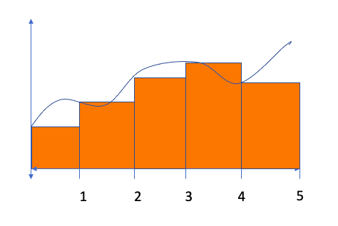
For a Left Riemann Sum, we’ll repeat the process, but use the left side of each rectangle to establish the height as shown below. This results in the following estimate:

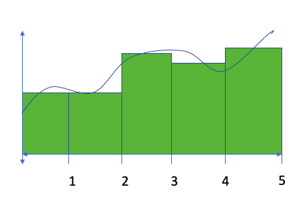
For a Midpoint Riemann Sum, we’ll find the height of each rectangle by using the height for the middle of each base as shown below. This results in the following estimation:

The final Riemann Sum is a trapezoidal sum. Recall that the area of a trapezoid is found by

In essence, we are multiplying the base by the average of the two heights. Using the original example function, that gives an estimate of

Note that in the examples above, each rectangle has the same base of length 1. In many problems, the bases will be of different lengths. Don’t forget to change the bases for each rectangle or trapezoid!
Finally, for some types of functions, it is possible to determine whether a particular kind of Riemann Sum will lead to an overestimate or an underestimate of the integral. For increasing functions, a Right Riemann Sum will always lead to an overestimate, because the right side of every rectangle will be higher than the actual function for that rectangle. Similarly, for decreasing functions, a Right Riemann Sum will always lead to an underestimate because the left side of every rectangle will be lower than the actual function for that rectangle.
These problems take a lot of practice, but once you commit the process for finding delta x and x sub i to memory, they become very doable. Good luck!
Browse Study Guides By Unit
👑Unit 1 – Limits & Continuity
🤓Unit 2 – Fundamentals of Differentiation
🤙🏽Unit 3 – Composite, Implicit, & Inverse Functions
👀Unit 4 – Contextual Applications of Differentiation
✨Unit 5 – Analytical Applications of Differentiation
🔥Unit 6 – Integration & Accumulation of Change
💎Unit 7 – Differential Equations
🐶Unit 8 – Applications of Integration
🦖Unit 9 – Parametric Equations, Polar Coordinates, & Vector-Valued Functions (BC Only)
♾Unit 10 – Infinite Sequences & Series (BC Only)
🧐Multiple Choice Questions (MCQ)
✍️Free Response Questions (FRQ)
📆Big Reviews: Finals & Exam Prep

© 2023 Fiveable Inc. All rights reserved.